Machine learning represents a transformative branch of artificial intelligence that enables systems to learn from data without explicit programming. Unlike traditional software that follows predefined rules, machine learning algorithms identify patterns in data and improve their performance through experience. This capability has revolutionized industries from healthcare to finance, powering everything from recommendation systems to autonomous vehicles.
At its core, machine learning mimics human learning by extracting patterns from data and making predictions or decisions based on those patterns. As data volumes grow exponentially, machine learning has become essential for uncovering insights that would be impossible to detect manually. This comprehensive guide explores the fundamental types of machine learning, essential algorithms, implementation processes, and practical deployment strategies.
Core Types of Machine Learning
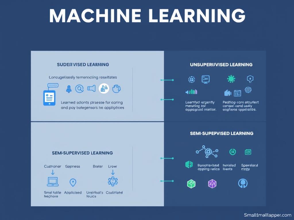
Machine learning approaches can be categorized into four main types, each suited to different kinds of problems and data availability. Understanding these fundamental categories is essential for selecting the right approach for your specific use case.
Supervised Learning
Supervised learning uses labeled training data to teach algorithms to predict outcomes or classify data into categories. The algorithm learns by comparing its predictions against known correct answers, adjusting its parameters to minimize errors.
Classification
Classification algorithms predict discrete categories or classes. For example, email spam filters use classification to determine whether a message is spam or legitimate based on features like sender information, content words, and formatting patterns.
Common applications include:
- Email spam detection
- Image recognition
- Medical diagnosis
- Customer churn prediction
Regression
Regression algorithms predict continuous numerical values rather than discrete categories. These models establish relationships between variables to forecast outcomes like prices, temperatures, or other quantitative measurements.
Common applications include:
- House price prediction
- Sales forecasting
- Temperature prediction
- Stock price analysis
Unsupervised Learning
Unsupervised learning works with unlabeled data, identifying patterns, structures, or relationships without predefined categories or outcomes. These algorithms discover hidden patterns that might not be apparent to human analysts.
Clustering
Clustering algorithms group similar data points together based on inherent similarities. These techniques help identify natural groupings within data without predefined categories.
Common applications include:
- Customer segmentation
- Anomaly detection
- Document categorization
- Image compression
Dimensionality Reduction
Dimensionality reduction techniques reduce the number of variables in a dataset while preserving essential information. This simplifies analysis, visualization, and model training.
Common applications include:
- Data visualization
- Feature extraction
- Noise reduction
- Computational efficiency improvement
Reinforcement Learning
Reinforcement learning involves an agent learning to make decisions by performing actions in an environment to maximize cumulative rewards. Unlike supervised learning, the algorithm isn’t trained on correct examples but learns through trial and error.
The agent interacts with its environment, observes the results of its actions, and adjusts its strategy to maximize long-term rewards. This approach is particularly effective for sequential decision-making problems.
Common applications include:
- Game playing (Chess, Go, video games)
- Autonomous vehicles
- Robotics control
- Resource management
- Recommendation systems
Semi-Supervised Learning
Semi-supervised learning combines elements of supervised and unsupervised learning, using a small amount of labeled data with a larger amount of unlabeled data. This approach is particularly valuable when labeling data is expensive or time-consuming.
Modern semi-supervised learning includes self-supervised learning, where the system generates its own labels from the data structure. This has become increasingly important in areas like natural language processing and computer vision.
Common applications include:
- Speech analysis
- Protein sequence classification
- Web content categorization
- Medical image analysis
Step-by-Step Machine Learning Pipeline
Implementing machine learning involves a structured pipeline from data preparation to model deployment. Each step is critical for building effective models that deliver accurate predictions.
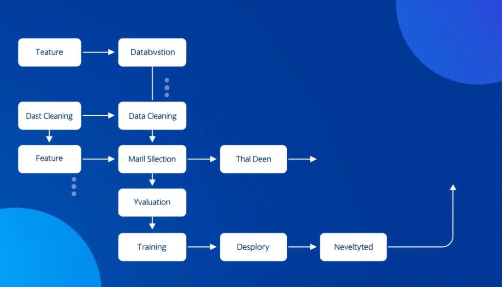
Data Cleaning
Raw data often contains inconsistencies, missing values, and errors that can significantly impact model performance. Data cleaning involves identifying and addressing these issues to create a reliable dataset for training.
Key Data Cleaning Steps:
- Handling missing values (imputation or removal)
- Removing duplicates
- Correcting structural errors
- Filtering outliers
- Standardizing text (case, formatting)
Here’s a Python example using pandas for basic data cleaning:
import pandas as pd
import numpy as np

# Load dataset
df = pd.read_csv('data.csv')

# Check for missing values
print(df.isnull().sum())

# Fill missing numerical values with mean
df['age'].fillna(df['age'].mean(), inplace=True)

# Fill missing categorical values with mode
df['category'].fillna(df['category'].mode()[0], inplace=True)

# Remove duplicates
df.drop_duplicates(inplace=True)

# Handle outliers using IQR method
Q1 = df['value'].quantile(0.25)
Q3 = df['value'].quantile(0.75)
IQR = Q3 - Q1
df = df[~((df['value']  (Q3 + 1.5 * IQR)))]
Feature Scaling
Many machine learning algorithms perform better when features are on similar scales. Feature scaling transforms numerical features to a standard range, preventing features with larger magnitudes from dominating the learning process.
Common scaling techniques include:
| Technique | Formula | Use Case |
| Min-Max Scaling (Normalization) | X’ = (X – Xmin) / (Xmax – Xmin) | When you need values in a specific range (0-1) |
| Standardization (Z-score) | X’ = (X – μ) / σ | When you need to handle outliers effectively |
| Robust Scaling | X’ = (X – median) / IQR | When data contains many outliers |
Python implementation using scikit-learn:
from sklearn.preprocessing import MinMaxScaler, StandardScaler, RobustScaler

# Min-Max Scaling
min_max_scaler = MinMaxScaler()
X_minmax = min_max_scaler.fit_transform(X)

# Standardization
standard_scaler = StandardScaler()
X_standardized = standard_scaler.fit_transform(X)

# Robust Scaling
robust_scaler = RobustScaler()
X_robust = robust_scaler.fit_transform(X)
Data Preprocessing in Python
Beyond cleaning and scaling, effective preprocessing includes feature engineering, encoding categorical variables, and splitting data for training and testing.
Categorical variable encoding is essential for converting text categories into numerical values that algorithms can process:
# One-hot encoding
df_encoded = pd.get_dummies(df, columns=['category', 'region'])

# Label encoding
from sklearn.preprocessing import LabelEncoder
label_encoder = LabelEncoder()
df['encoded_category'] = label_encoder.fit_transform(df['category'])

# Train-test split
from sklearn.model_selection import train_test_split
X = df.drop('target', axis=1)
y = df['target']
X_train, X_test, y_train, y_test = train_test_split(X, y, test_size=0.2, random_state=42)
Supervised Learning Deep Dive
Supervised learning algorithms form the foundation of many practical machine learning applications. Let’s explore the most important algorithms, their characteristics, and use cases.
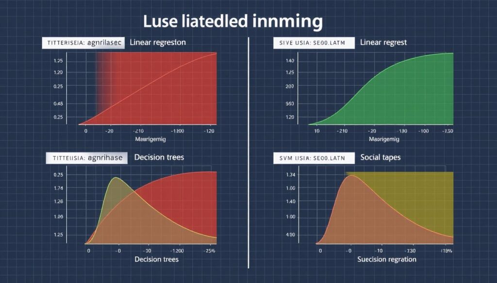
Linear and Logistic Regression
Linear Regression
Linear regression models the relationship between a dependent variable and one or more independent variables using a linear equation. It’s the foundation of many predictive models and provides interpretable results.
The basic form is: y = β₀ + β₁x₁ + β₂x₂ + … + βₙxₙ + ε
Where:
- y is the dependent variable
- x₁, x₂, …, xₙ are independent variables
- β₀, β₁, β₂, …, βₙ are coefficients
- ε is the error term
Logistic Regression
Despite its name, logistic regression is a classification algorithm that estimates the probability of an instance belonging to a particular class. It uses the logistic function to transform linear predictions into probability values between 0 and 1.
The logistic function is: P(y=1) = 1 / (1 + e^(-z))
Where z = β₀ + β₁x₁ + β₂x₂ + … + βₙxₙ
Common applications include:
- Credit scoring
- Medical diagnosis
- Marketing conversion prediction
Decision Trees and Random Forests
Decision Trees
Decision trees create a model that predicts the value of a target variable by learning simple decision rules inferred from data features. They’re intuitive, easy to visualize, and can handle both numerical and categorical data.
Key advantages:
- Highly interpretable
- Require minimal data preparation
- Can handle both numerical and categorical data
- Automatically handle feature interactions
Random Forests
Random forests are an ensemble learning method that constructs multiple decision trees during training and outputs the class that is the mode of the classes (classification) or mean prediction (regression) of the individual trees.
Key advantages:
- Higher accuracy than individual decision trees
- Reduced risk of overfitting
- Built-in feature importance evaluation
- Handles high-dimensional data effectively
 30?’, ‘Income > 50K?’) and classification outcomes at leaf nodes. Use a blue and green color scheme with clean lines and readable text.”>
Support Vector Machines and k-NN
Support Vector Machines (SVM)
SVMs find the hyperplane that best separates classes in feature space, maximizing the margin between the closest points (support vectors) from each class. They’re effective in high-dimensional spaces and with clear margins of separation.
Key advantages:
- Effective in high-dimensional spaces
- Memory efficient (uses subset of training points)
- Versatile through different kernel functions
- Robust against overfitting in high-dimensional spaces
k-Nearest Neighbors (k-NN)
k-NN is a non-parametric method that classifies objects based on the majority class among their k nearest neighbors in the feature space. It’s intuitive and makes no assumptions about the underlying data distribution.
Key advantages:
- Simple implementation
- Adapts easily as new training data becomes available
- No training phase (lazy learning)
- Naturally handles multi-class problems
Naïve Bayes and Ensemble Methods
Naïve Bayes
Naïve Bayes classifiers apply Bayes’ theorem with the “naïve” assumption of conditional independence between features. Despite this simplification, they often perform surprisingly well, especially with text classification.
Variants include:
- Gaussian Naïve Bayes (for continuous data)
- Multinomial Naïve Bayes (for discrete counts, like word frequencies)
- Bernoulli Naïve Bayes (for binary features)
Ensemble Learning
Ensemble methods combine multiple models to improve performance beyond what any single model could achieve. The two main approaches are:
Bagging (Bootstrap Aggregating): Trains multiple instances of the same model on different subsets of data and averages their predictions (e.g., Random Forest).
Boosting: Trains models sequentially, with each model focusing on the errors of previous models (e.g., AdaBoost, Gradient Boosting).
| Algorithm | Strengths | Weaknesses | Ideal Use Cases |
| Linear Regression | Simple, interpretable, fast | Assumes linear relationship, sensitive to outliers | Price prediction, trend analysis |
| Logistic Regression | Probabilistic output, interpretable | Assumes linear decision boundary | Binary classification, risk assessment |
| Decision Trees | Intuitive, handles mixed data types | Can overfit, unstable | Rule-based systems, feature importance analysis |
| Random Forest | Robust, handles high dimensionality | Less interpretable, computationally intensive | Complex classification, feature selection |
| SVM | Effective in high dimensions, memory efficient | Sensitive to parameter tuning, slower training | Text classification, image recognition |
| k-NN | Simple, no training required | Slow prediction, requires feature scaling | Recommendation systems, anomaly detection |
Unsupervised Learning Techniques
Unsupervised learning discovers hidden patterns in unlabeled data, making it valuable for exploratory data analysis and feature discovery. Let’s examine the key techniques and their applications.
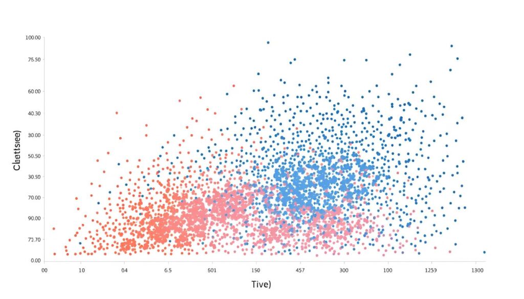
Clustering Algorithms
Clustering algorithms group similar data points together based on distance or density measures. These techniques are widely used for customer segmentation, anomaly detection, and data preprocessing.
K-Means Clustering
K-means partitions data into K distinct clusters by minimizing the within-cluster variance. It’s efficient and works well with large datasets but requires specifying the number of clusters in advance.
The algorithm:
- Initialize K cluster centers
- Assign each point to the nearest center
- Recalculate centers as the mean of assigned points
- Repeat steps 2-3 until convergence
DBSCAN
Density-Based Spatial Clustering of Applications with Noise (DBSCAN) groups points that are closely packed together while marking points in low-density regions as outliers.
Key advantages:
- Doesn’t require specifying number of clusters
- Can find arbitrarily shaped clusters
- Robust to outliers
- Works well with spatial data
Hierarchical Clustering
Hierarchical clustering builds a tree of clusters, providing a multi-level view of data organization. It can be agglomerative (bottom-up) or divisive (top-down).
Key advantages:
- Creates intuitive visualization (dendrogram)
- Doesn’t require specifying number of clusters
- Captures hierarchical relationships
- Works well with small to medium datasets
# K-means clustering example
from sklearn.cluster import KMeans
import numpy as np

# Create sample data
X = np.array([[1, 2], [1, 4], [1, 0], [4, 2], [4, 4], [4, 0]])

# Create and fit the model
kmeans = KMeans(n_clusters=2, random_state=0).fit(X)

# Get cluster labels and centers
labels = kmeans.labels_
centers = kmeans.cluster_centers_

# Predict new data
new_data = np.array([[0, 0], [5, 5]])
kmeans.predict(new_data)
Dimensionality Reduction
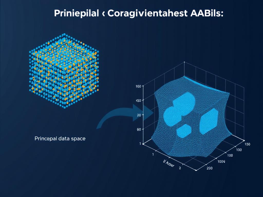
Dimensionality reduction techniques transform high-dimensional data into a lower-dimensional space while preserving essential information. These methods improve computational efficiency, reduce noise, and enable visualization of complex datasets.
Principal Component Analysis (PCA)
PCA transforms data into a new coordinate system where the greatest variance lies on the first coordinate (principal component), the second greatest variance on the second coordinate, and so on.
Key applications:
- Feature extraction
- Data compression
- Visualization of high-dimensional data
- Noise filtering
t-SNE
t-Distributed Stochastic Neighbor Embedding (t-SNE) is particularly effective for visualizing high-dimensional data by giving each datapoint a location in a two or three-dimensional map.
Key advantages:
- Preserves local structure of data
- Reveals clusters at multiple scales
- Excellent for visualization
- Works well with non-linear relationships
Association Rule Mining
Association rule mining discovers interesting relationships between variables in large databases. It’s widely used in market basket analysis to identify items frequently purchased together.
Apriori Algorithm
The Apriori algorithm identifies frequent itemsets and generates association rules with confidence above a minimum threshold. It uses the principle that if an itemset is frequent, then all of its subsets must also be frequent.
Key metrics:
- Support: Frequency of an itemset in the dataset
- Confidence: Likelihood of item Y being purchased when item X is purchased
- Lift: Ratio of observed support to expected support if X and Y were independent
# Apriori algorithm example using mlxtend
from mlxtend.frequent_patterns import apriori, association_rules
import pandas as pd

# Sample transaction data
data = {
    'Transaction': [1, 1, 1, 2, 2, 3, 3, 3, 3],
    'Item': ['Bread', 'Milk', 'Eggs', 'Bread', 'Milk', 'Bread', 'Milk', 'Eggs', 'Butter']
}
df = pd.DataFrame(data)

# Convert to one-hot encoded format
basket = df.pivot_table(index='Transaction', columns='Item', aggfunc=lambda x: 1, fill_value=0)

# Generate frequent itemsets
frequent_itemsets = apriori(basket, min_support=0.5, use_colnames=True)

# Generate association rules
rules = association_rules(frequent_itemsets, metric="confidence", min_threshold=0.7)
print(rules)
Reinforcement Learning Explained
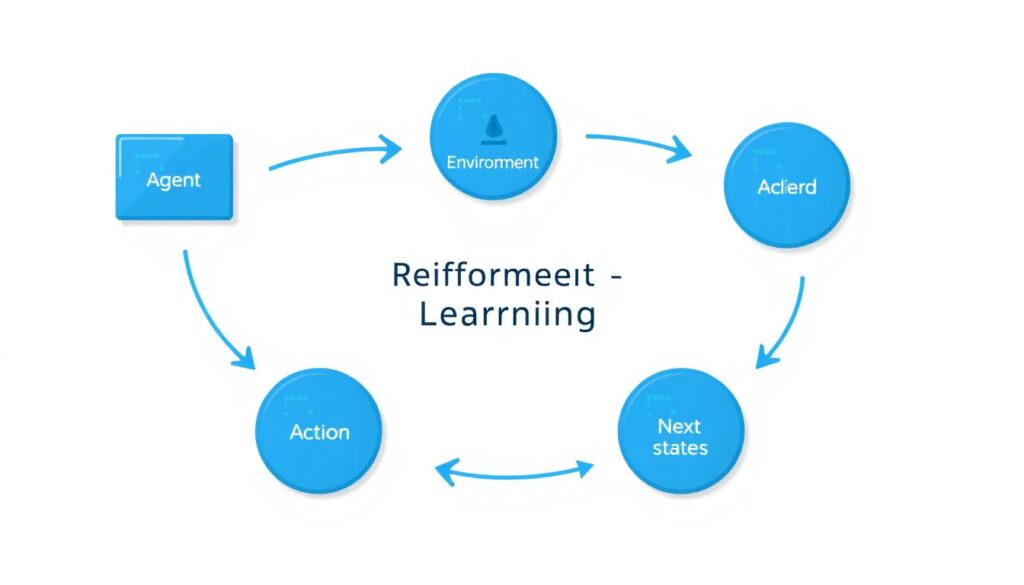
Reinforcement learning enables an agent to learn optimal behavior through interactions with an environment, receiving rewards or penalties based on its actions. This approach has achieved remarkable success in games, robotics, and resource management.
Key Components
Agent
The agent is the learner or decision-maker that interacts with the environment. It observes states, takes actions, and receives rewards or penalties.
Environment
The environment represents everything the agent interacts with. It provides states and rewards in response to the agent’s actions.
Policy
The policy is the agent’s strategy for selecting actions based on the current state. It maps states to actions and is what the agent aims to optimize.
Model-Based Methods
Model-based reinforcement learning methods build an internal model of the environment to plan and make decisions. These approaches can be more sample-efficient but require accurate environment modeling.
Markov Decision Processes (MDPs)
MDPs provide a mathematical framework for modeling decision-making in situations where outcomes are partly random and partly under the control of a decision-maker. An MDP consists of:
- A set of states S
- A set of actions A
- Transition probabilities P(s’|s,a)
- Reward function R(s,a,s’)
- Discount factor γ (0 ≤ γ ≤ 1)
Bellman Equation
The Bellman equation is a fundamental concept in reinforcement learning that expresses the relationship between the value of a state and the values of its successor states:
V(s) = maxa [R(s,a) + γ Σs’ P(s’|s,a) V(s’)]
Where V(s) is the value of state s, representing the expected cumulative reward starting from that state and following the optimal policy.
Model-Free Methods
Model-free methods learn directly from interactions with the environment without building an explicit model. They’re more adaptable to complex environments but may require more samples to learn effectively.
Q-Learning
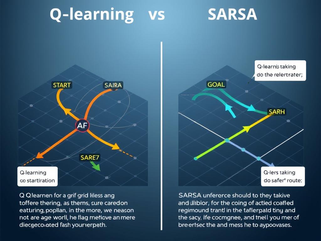
Q-learning is a value-based approach that learns the value of action a in state s, denoted as Q(s,a). It updates Q-values using the Bellman equation without requiring a model of the environment.
The Q-value update rule is:
Q(s,a) ← Q(s,a) + α[r + γ maxa’ Q(s’,a’) – Q(s,a)]
Where:
- α is the learning rate
- γ is the discount factor
- r is the immediate reward
- s’ is the next state
SARSA
SARSA (State-Action-Reward-State-Action) is an on-policy algorithm that updates Q-values based on the action actually taken in the next state, rather than the maximum possible value.
The update rule is:
Q(s,a) ← Q(s,a) + α[r + γ Q(s’,a’) – Q(s,a)]
Key differences from Q-learning:
- Uses the actual next action a’ (on-policy)
- Often more conservative in risky environments
- Converges to the optimal policy more slowly
Deep Reinforcement Learning
Deep reinforcement learning combines reinforcement learning with deep neural networks to handle high-dimensional state spaces. This approach has achieved breakthrough results in complex domains like game playing and robotics.
Deep Q-Networks (DQN)
DQN uses deep neural networks to approximate the Q-function, enabling reinforcement learning in environments with high-dimensional state spaces. Key innovations include:
- Experience replay: Storing and randomly sampling past experiences to break correlations between sequential samples
- Target networks: Using a separate network for generating targets to stabilize training
- Convolutional layers: Processing visual input effectively
Semi-Supervised Learning Approaches
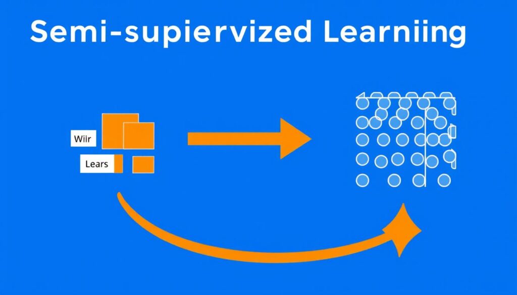
Semi-supervised learning leverages both labeled and unlabeled data to improve model performance, especially when labeled data is scarce or expensive to obtain. This approach has gained significant importance in recent years with the rise of self-supervised techniques.
Key Concepts
Semi-Supervised Classification
Semi-supervised classification uses a small amount of labeled data to guide the classification of a larger unlabeled dataset. Common approaches include:
- Self-training: The model iteratively labels unlabeled data and retrains using its own predictions
- Co-training: Multiple models train on different views of the data and teach each other
- Graph-based methods: Leverage the relationship between data points to propagate labels
Self-Supervised Learning
Self-supervised learning generates supervisory signals from the data itself by creating “pretext tasks” that don’t require manual labeling. The model learns useful representations that can be fine-tuned for downstream tasks.
Common pretext tasks include:
- Predicting masked or missing parts of the input
- Predicting the relative position of image patches
- Colorizing grayscale images
- Predicting the next word or sentence in text
Few-Shot Learning
Few-shot learning aims to train models that can generalize to new classes with only a few examples. This approach is particularly valuable when collecting large labeled datasets is impractical.
Key techniques include:
- Meta-learning: “Learning to learn” by training on a variety of tasks
- Siamese networks: Learning similarity metrics between examples
- Prototypical networks: Learning class prototypes and classifying based on distance
- Transfer learning: Adapting pre-trained models to new tasks with limited data
# Simple self-training example
from sklearn.semi_supervised import SelfTrainingClassifier
from sklearn.svm import SVC
import numpy as np

# Create labeled and unlabeled data
X_labeled = np.array([[0, 1], [1, 0], [0, 0], [1, 1]])
y_labeled = np.array([0, 0, 1, 1])
X_unlabeled = np.array([[0.1, 0.9], [0.9, 0.1], [0.1, 0.1], [0.9, 0.9]])

# Combine data (unlabeled has -1 as label)
X_combined = np.vstack((X_labeled, X_unlabeled))
y_combined = np.append(y_labeled, [-1, -1, -1, -1])

# Create and train self-training classifier
base_clf = SVC(probability=True, kernel='rbf')
self_training_clf = SelfTrainingClassifier(base_clf)
self_training_clf.fit(X_combined, y_combined)

# Predict on new data
X_new = np.array([[0.2, 0.8], [0.8, 0.2]])
predictions = self_training_clf.predict(X_new)
print(predictions)
Deploying Machine Learning Models
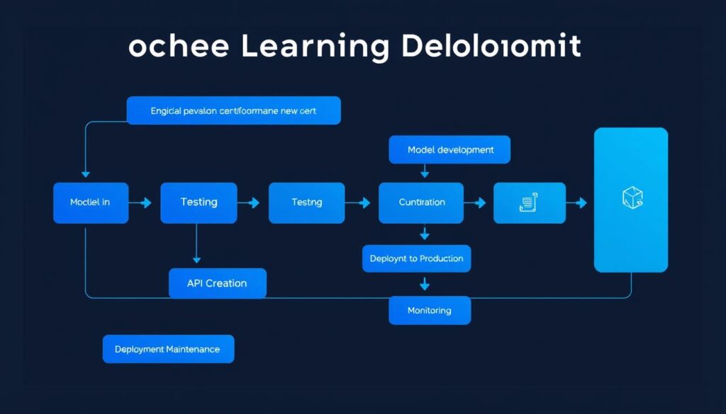
Deploying machine learning models transforms theoretical algorithms into practical applications that deliver value. Effective deployment requires careful planning, appropriate tools, and ongoing monitoring.
Web App Deployment
Web applications provide an accessible interface for users to interact with machine learning models. Several frameworks simplify the process of creating and deploying ML-powered web apps.
Streamlit
Streamlit is a Python library that makes it easy to create custom web apps for machine learning models with minimal front-end development experience.
Key features:
- Simple Python-based interface
- Rapid prototyping capabilities
- Interactive widgets for user input
- Easy integration with data visualization libraries
Gradio
Gradio allows you to quickly create customizable UI components for machine learning models, with a focus on making models demo-ready.
Key features:
- Simple API for creating interfaces
- Support for various input/output types
- Easy sharing of demos via temporary links
- Integration with Hugging Face Spaces
# Streamlit example
import streamlit as st
import pandas as pd
import numpy as np
from sklearn.ensemble import RandomForestClassifier

# Load and train model (in practice, load pre-trained model)
@st.cache_data
def load_model():
    # Simulate model training or loading
    model = RandomForestClassifier()
    # In practice: model.load("model.pkl") or similar
    return model

model = load_model()

# Create web interface
st.title("Machine Learning Model Deployment")
st.write("Enter values to get predictions")

# Input widgets
feature1 = st.slider("Feature 1", 0.0, 10.0, 5.0)
feature2 = st.slider("Feature 2", 0.0, 10.0, 5.0)
feature3 = st.selectbox("Feature 3", options=["Option A", "Option B", "Option C"])

# Convert categorical to numerical
feature3_encoded = 0 if feature3 == "Option A" else 1 if feature3 == "Option B" else 2

# Make prediction when button is clicked
if st.button("Predict"):
    input_data = np.array([[feature1, feature2, feature3_encoded]])
    prediction = model.predict(input_data)
    st.success(f"Prediction: {prediction[0]}")
API Development
APIs (Application Programming Interfaces) allow machine learning models to be integrated into larger applications and systems. They provide a standardized way to send data to and receive predictions from models.
Flask
Flask is a lightweight web framework for Python that’s popular for creating ML model APIs due to its simplicity and flexibility.
Key features:
- Minimal and flexible framework
- Easy to understand and implement
- Good for simple to moderate complexity APIs
- Extensive documentation and community support
FastAPI
FastAPI is a modern, high-performance web framework for building APIs with Python, based on standard Python type hints.
Key features:
- High performance (on par with NodeJS and Go)
- Automatic interactive documentation
- Data validation with Pydantic
- Asynchronous support
# FastAPI example
from fastapi import FastAPI
from pydantic import BaseModel
import pickle
import numpy as np

# Define input data model
class ModelInput(BaseModel):
    feature1: float
    feature2: float
    feature3: int

# Initialize FastAPI
app = FastAPI(title="ML Model API")

# Load pre-trained model
model = pickle.load(open("model.pkl", "rb"))

@app.post("/predict")
async def predict(input_data: ModelInput):
    # Convert input to numpy array
    input_array = np.array([[
        input_data.feature1,
        input_data.feature2,
        input_data.feature3
    ]])

    # Make prediction
    prediction = model.predict(input_array)
    probability = model.predict_proba(input_array).max()

    # Return prediction
    return {
        "prediction": int(prediction[0]),
        "probability": float(probability)
    }
Cloud Deployment
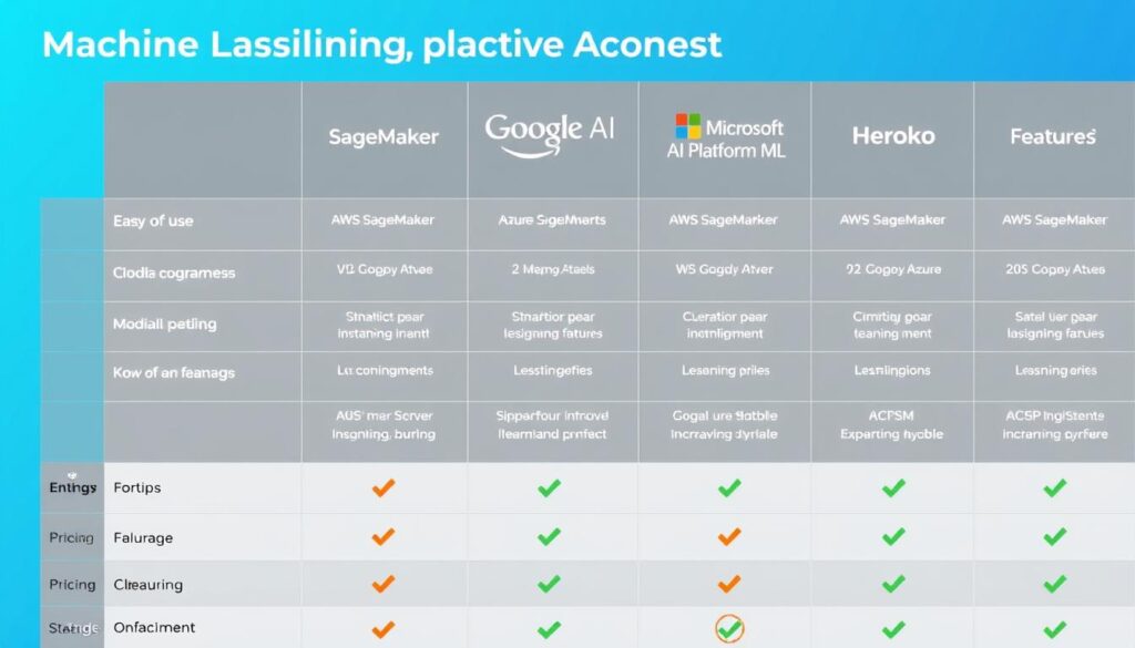
Cloud platforms provide scalable infrastructure for deploying machine learning models, with options ranging from fully managed services to customizable containers.
Heroku
Heroku is a platform-as-a-service (PaaS) that enables developers to build, run, and operate applications entirely in the cloud.
Key advantages:
- Simple deployment process
- Free tier for small applications
- Automatic scaling capabilities
- Supports multiple programming languages
AWS SageMaker
Amazon SageMaker is a fully managed service that provides tools to build, train, and deploy machine learning models at scale.
Key advantages:
- End-to-end ML workflow support
- Automatic scaling for inference
- Built-in model monitoring
- Integration with other AWS services
Google AI Platform
Google AI Platform provides tools for every step of the ML workflow, from data preparation to model deployment and monitoring.
Key advantages:
- Integration with TensorFlow and other frameworks
- Scalable training and prediction
- Support for custom containers
- Automated ML capabilities
Monitoring and Maintenance
Deploying a model is just the beginning. Ongoing monitoring and maintenance are essential to ensure models continue to perform well as data distributions change over time.
Key monitoring aspects include:
- Performance metrics: Tracking accuracy, precision, recall, and other relevant metrics
- Data drift: Detecting changes in input data distribution
- Concept drift: Identifying changes in the relationship between inputs and outputs
- Resource utilization: Monitoring computational resources and response times
- User feedback: Collecting and analyzing user interactions and feedback
Conclusion
Machine learning has evolved from a theoretical concept to a transformative technology that powers countless applications across industries. By understanding the core types of machine learning, essential algorithms, and deployment strategies, you can harness this powerful technology to solve complex problems and create innovative solutions.
The journey from data to deployed model involves multiple steps, each requiring careful consideration and expertise. From selecting the right algorithm for your problem to preparing data, training models, and deploying them in production environments, every stage contributes to the ultimate success of your machine learning project.
As machine learning continues to advance, staying current with new techniques and best practices will be essential. The field is rapidly evolving, with innovations in areas like self-supervised learning, reinforcement learning, and model deployment constantly expanding the possibilities of what machine learning can achieve.
